Note: this article was co-written with L&R’s Michael LeClair.

The FCC requires that every FM station perform a series of measurements of the broadcast spectrum every time any change is made the baseband of the signal. Specifically, you have to measure Occupied Bandwidth, or OBW, and you have to ensure your harmonics are within tolerance. These measurements are referred to, broadly, as “Equipment Performance Measurements” or “EPM’s.”

The actual text of 47 CFR § 73.1590 reads as follows. I’ve bolded the parts that apply specifically to FM radio stations, and strikethrough’d some parts not relevant to FM.

(a) The licensee of each AM, FM, TV and Class A TV station, except licensees of Class D non-commercial educational FM stations authorized to operate with 10 watts or less output power, must make equipment performance measurements for each main transmitter as follows:

(1) Upon initial installation of a new or replacement main transmitter.

(2) Upon modification of an existing transmitter made under the provisions of § 73.1690, Modification of transmission systems, and specified therein.

(3) Installation of AM stereophonic transmission equipment pursuant to § 73.128.

(4) Installation of FM subcarrier or stereophonic transmission equipment pursuant to § 73.295, § 73.297, § 73.593 or § 73.597.

(5) [Reserved]

(6) Annually, for AM stations, with not more than 14 months between measurements.

(7) When required by other provisions of the rules or the station license.

(b) Measurements for spurious and harmonic emissions must be made to show compliance with the transmission system requirements of § 73.44 for AM stations; § 73.317 for FM stations and § 73.687 for TV stations. Measurements must be made under all conditions of modulation expected to be encountered by the station whether transmitting monophonic or stereophonic programs and providing subsidiary communications services.

(c) TV visual equipment performance measurements must be made with the equipment adjusted for normal program operation at the transmitter antenna sampling port to yield the following information:

(1) [Reserved]

(2) Data showing that the waveform of the transmitted signal conforms to that specified by the standards for TV transmissions.

(3) [Reserved]

(4) Data showing envelope delay characteristics of the radiated signal.

(5) Data showing the attenuation of spurious and harmonic radiation, if, after type acceptance, any changes have been made in the transmitter or associated equipment (filters, multiplexer, etc.) which could cause changes in its radiation products.

(d) The data required by paragraphs (b) and (c) of this section, together with a description of the equipment and procedure used in making the measurements, signed and dated by the qualified person(s) making the measurements, must be kept on file at the transmitter or remote control point for a period of 2 years, and on request must be made available during that time to duly authorized representatives of the FCC.

[47 FR 8589, Mar. 1, 1982, as amended at 51 FR 18450, May 20, 1986; 65 FR 30004, May 10, 2000; 89 FR 7255, Feb. 1, 2024]

L&R recently performed Equipment Performance Measurements for newly licensed WMVC, 91.5FM, Edgartown, MA and broadcasting from the rooftop of the Winnetu Resort in Katama, MA. This is right on the ocean’s edge at the southeastern corner of Martha’s Vineyard…an offshore island.

This is, in many ways, an easy station to do an EPM for:

1. The station has a brand-new high-quality FM transmitter (Nautel VX300).
2. The station isn’t running HD Radio, nor any SCA/subcarriers beyond the stereo pilot and RDS.
3. There’s no other FM broadcast stations nearby. In fact: for quite a few directions, there’s no FM broadcast stations for over a thousand miles.

We used an Agilent E4402B spectrum analyzer, or “SA.” All we had to do was bring a 10ft long cable with BNC connectors and a few adapters to mate the Nautel’s RF sample port with the SA input.

Step 1: Set your FCC mask & prep the spectrum analyzer

Before you do any measurements, you need to create a “limit mask” that displays on your SA screen. This provides a visual representation of the requirements of § 73.317 as follows for standard FM broadcast:

• Between 120 and 240 kHz off-carrier, signal must be attenuated -25dB below reference.
• Between 240 and 600 kHz off-carrier, signal must be attenuated -35dB below reference.
• Beyond 600 kHz off-carrier, signal must be attenuated -80dB below reference, or 43 + 10 Log¹⁰ (Power, in watts) dB below the unmodulated carrier. (whichever is lesser attenuation, but usually one will end up using -80dB; in our case we could use the other formula because our TPO (260w) is so low: 43 + 10 Log¹⁰ (260) dB = 67.14 dB
• If HD Radio is deployed, there is a more complex Limit Mask that should be used to reflect the transmission requirements of this system which generates sideband carriers out to 200 kHz away from the carrier frequency.

Your display should be set to 10dB per division, logarithmic Scale type, and about 1.6 MHz Span to start with. You’ll change that to 1.0 MHz for the actual measurements, but 1.6 is good for the reference level setting in step 2.

Step 2: Set your reference level

SAFETY FIRST

Before attaching a sample line from a transmitter or RF system you need think about what the expected level should be. For this simple system, with no other radiating RF sources on the rooftop, it was safe to assume the sample feed would not be at a dangerous level to the analyzer. But in general, it makes sense to start with an attenuator or two inserted into the sample line before the SA.

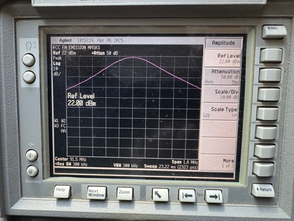
We began by setting the center frequency of the signal to be measured (91.5 MHz in WMVC’s case) and resolution bandwidth (RBW) around 1-3 kHz. Make the Video Bandwidth (VBW) track the RBW if it’s not automatic. You want 10dB of signal strength per division on the amplitude setting.

If you are in a high RF area with lots of radiating antennas, start by setting the span fairly wide (maybe 400 MHz). This is just in case there is something with a lot of energy nearby that could couple into the antenna and back down into the SA. This wide span will allow you to see the whole FM band and up into the TV band. With this wide a span the trace will move very slowly. To speed it up you can increase the RBW as needed.

Once you have determined it’s safe to keep measuring, reduce the span to around 1.6 MHz for a standard FM station. Set the RBW to 3 kHz. You should see the FM carrier for the station under test.

The trace display should clear after every sweep of the analyzer. This will appear as a variable line of what looks like noise and an FM carrier with modulation at the center frequency.

GET IT RIGHT

Setting the amplitude accurately is the most important step to get right. All the other measurements depend on it. I use a technique taught to me by David Maxson, a long time RF consultant in our area.

Start changing the RBW setting to 300 kHz on the SA. See the picture below of what to expect. You’ll still see some small variations in the display, but with a RBW this high you won’t be able to make out the individual signal sidebands which have a maximum modulation of 75 kHz. In effect, you’ve changed the display to show you a very smoothed curved of the signal power. The goal is to set the signal amplitude for the transmitter test to just touch the top of the display grid. Do NOT use an automatic level adjust function- this will not work for these measurements- you have to do it manually to preserve the later tests of harmonics.

Note the reference level; in our case it’s 22dBm (shown on the screen in the upper left corner. 1 dBm corresponds to 1 milliwatt, or 0.001 watts.

As a pop quiz, how much power is in a +22 dBm signal? Would this be dangerous to our analyzer which has a maximum rating of 2 watts of power? [answer is at end of this article]

Step 3: Occupied Bandwidth (OBW)

Next up is the OBW measurement. This ensures your signal isn’t causing undesired/illegal interference to any adjacent-channel signals.

Bring your RBW and VBW down to 1 kHz (your sweep will slow to about 1 to 1.5 sec each). Span can be anywhere from 800 kHz to 1.2 MHz, so we chose 1 MHz. Nice, round number.

NOISES OUT

A spectrum analyzer is showing you the instantaneous signal level at roughly 2500 points across the horizontal span. It’s important to consider this when making measurements that require a noise floor down to – 80 dB below the carrier peak power (aka unmodulated carrier power). It’s also important to understand the impact of RBW on the displayed noise level of the analyzer.

The lower the RBW, the less noise (or signal) power will be included in each display point. However, this takes a lot more processing power for the analyzer to calculate these values as you reduce the RBW. This is why you would not simply set the RBW to 1 Hz to get the lowest noise. Each scan would take an hour to complete. The goal is to find a tradeoff point where the scan is being displayed with reasonable speed, but the noise floor is maintained at – 100 dB in the analyzer. This usually corresponds to an RBW of around 100 to 300 Hz. I like to see the noise floor at the -100 dB level as it makes it easy to see if the measured signal under test is meeting the very difficult standard of -80 dB below carrier power at all points along the scan as defined by the limit mask.

KNOW YOUR LIMITS

For OBW you should set the analyzer trace to peak hold. We ran the test for about five minutes to make sure there were no infrequent peaks that exceeded the mask limit. See the photo below.

The mask limit is the white line that defines the maximum limit of energy for our standard FM station in terms of distance from the carrier frequency. Note how the limit line matches the top of the analyzer grid in the region of the center frequency. As we move away from the center frequency the limit mask becomes progressively more strict. Even though the standard is not as strict for low power stations, I prefer to start with the expectation the amplifier should -80 dB below the limit mask at both edges.

Most modern amplifiers should be able to achieve this. The yellow line is peak-hold, the purple is an instantaneous value. The bottom most grid line corresponds to -100 dB. The grey line is our aforementioned FCC mask as determined by § 73.317.

As you can see, this nice, new transmitter is very much in compliance with the rules. That yellow line doesn’t even come close to exceeding the limits at any frequency. Note the peak hold yellow line is exceeding the -80 dB standard which is the second horizontal grid line on the display.

A couple of other things to note on the analyzer. In the lower right corner of the display you can see the Span (1 MHz), the Sweep time (1.288 secs) and the total number of points (2323). While this measurement is perfectly acceptable, if we wanted to get an even more precise measurement of the noise floor we could change the RBW down to 300 Hz. I often do this when measuring HD Radio signals but it does demand some patience since the sweep time goes up by a factor of about 50. But the instantaneous signal trace will nicely decline to just about -100dB for maximum clarity…if you’ve got the time to wait for it.

Step 4: Harmonics

There’s no such thing as an RF signal without harmonics, which are just multiples of the original carrier. Ergo: the harmonics for WMVC are just 91.5 MHz multiplied by a given integer number:

• “First harmonic” = the Carrier Frequency, or 91.5 MHz
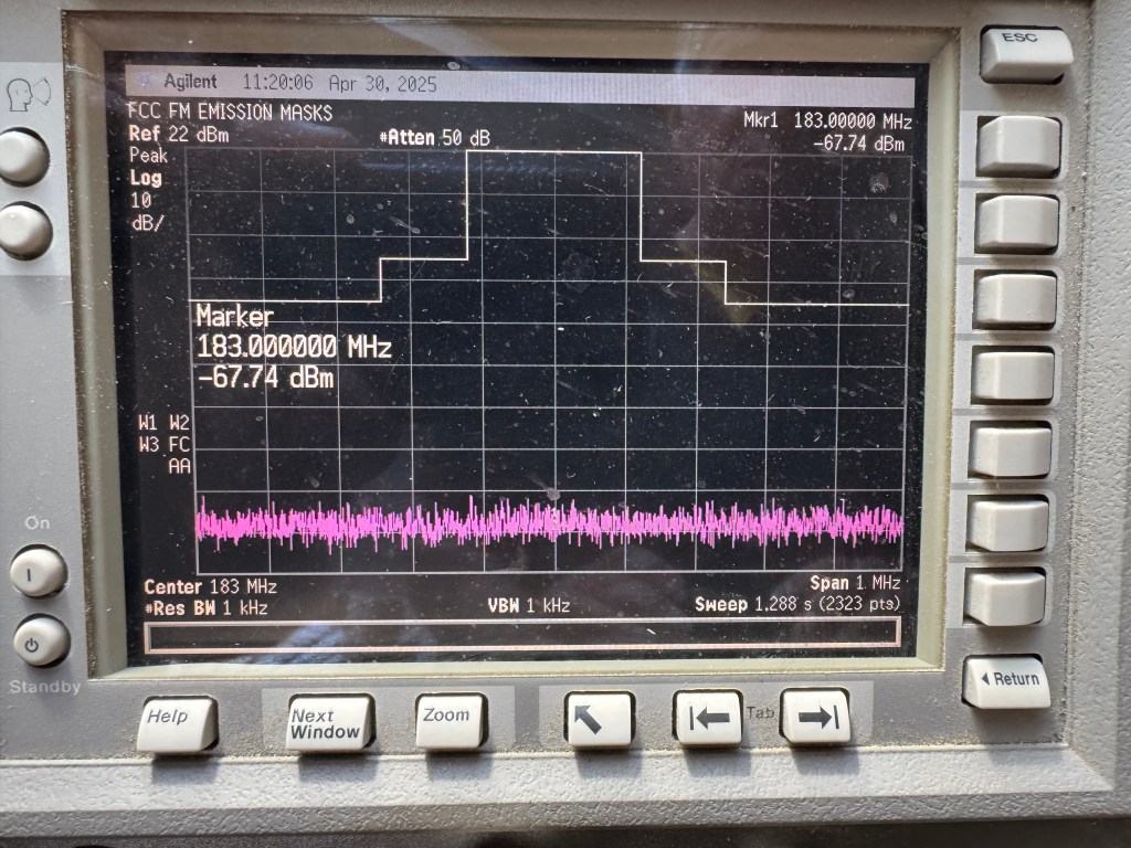
• Second harmonic is 91.5 MHz x 2 = 183 MHz
• Third harmonic is 91.5MHz x 3 = 274.5 MHz
• Fourth harmonic is 91.5 MHz x 4 = 366.0 MHz

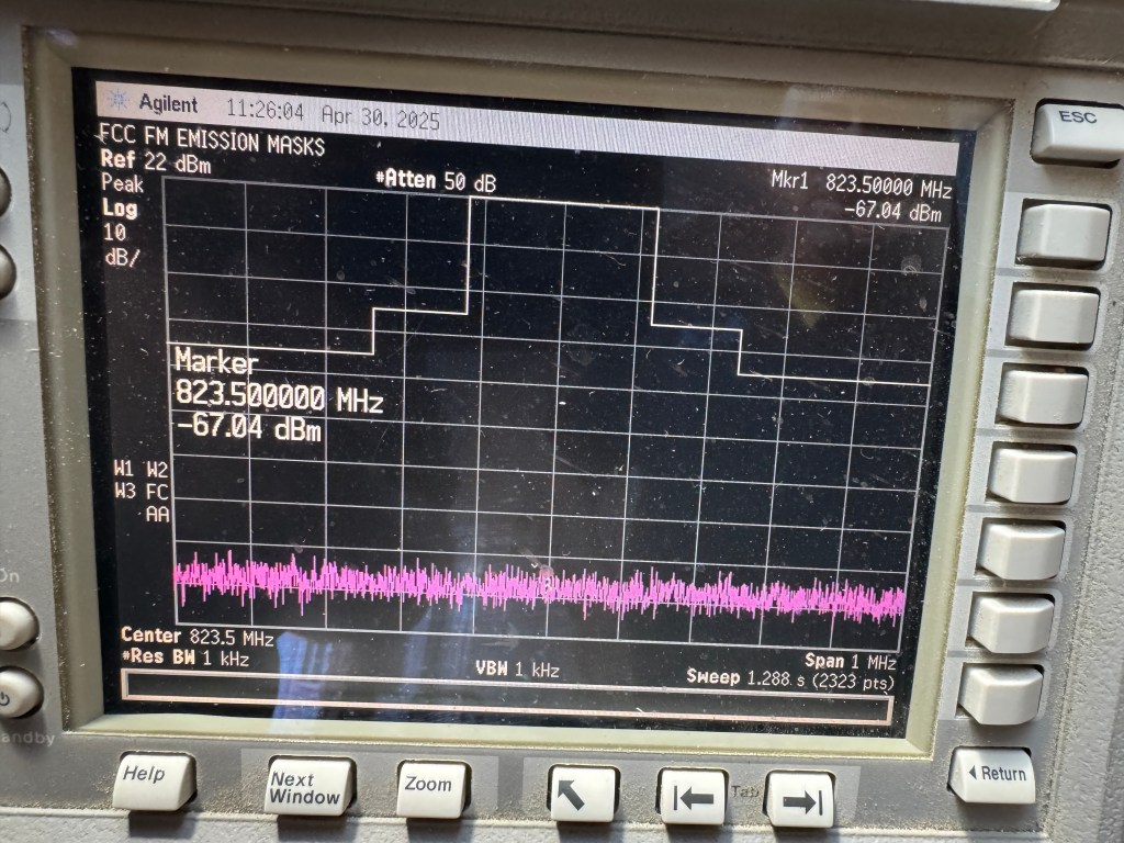
And so on and so forth out to the ninth harmonic; there’s no reason to measure any further than that. Due to how physics works, each greater harmonic is typically lower in power than previous harmonic. Accordingly, the second harmonic is usually the most troublesome as it will have the most power.

In modern times, the higher harmonics…seventh, eighth and ninth…are sometimes more sensitive because they tend to be in frequency bands where wireless carriers operate, and they operate at very low powers; nearly in the noise floor. So your higher harmonics need to be very clean and very minimized lest AT&T or Verizon come after you with the FCC enforcement bureau.

All harmonic spurs are supposed to be at least 80dB below an unmodulated carrier. The analyzer should be set up with the exact same span and amplitude settings as when we took the first images. Then the center frequency is moved up to each harmonic in turn until all have been read. I like to place a marker at the center frequency to get a very accurate measurement of the level. Modulation should be turned off during this measurement.

KEEP A LEVEL HEAD

You’ll note in the images below that the markers on the harmonics’ frequencies are only -67dB or so. What’s the deal? Don’t they need to be -80 dB?? The deal is our reference level, taken back in Step 2! You have to add the attenuation of the reference level (22dBm) to the measured level to get the actual reading. So in the second harmonic measurement, the actual reading is -89.74dB. In the ninth, it’s -89.04dB. Well below the required threshold.

You can also intuit this by, again, remembering the vertical axis is 10dB per division, and the purple line is below the 8th horizontal line on the screen…meaning it’s below -80dB.

That’s important because it’s possible you’ll see parts of the spectrum that aren’t on the harmonic frequency…but still are above the -80dB threshold. What does that mean? Most likely it’s the presence of some other RF source (like a nearby cell tower) getting into your transmitting antenna and causing some kind of interaction inside your transmitter. That’s not necessarily against the rules, but it does mean you have to ensure that it’s not a problem with your transmitter. Usually the best way to check that is to disconnect your transmitter from the antenna and operate into a dummy load to get a clear display of the spectrum . That wasn’t necessary in WMVC’s case, but it often can be for many stations that broadcast from a tower or building with other sources of RF on it.

I didn’t include screen captures of all the harmonic measurements for WMVC, 2nd through 9th, but we did take the measurements. And we included them in our final report.

Step 5: Write it all up for your EPM report

As § 73.1590 notes in section (d), you must create a report that documents:

1. The actual measurements themselves.
2. Description of the equipment & procedures used in making the measurements.
3. Signature of the qualified person(s) making the measurements.

In modern times this has never been easier, as you can use a smartphone to take pictures of the spectrum analyzer display as you go, and then insert the images into your Word document for the report.

ADD YOUR JOHN HANCOCK

Once the report is finished, you print it out, sign it, and keep it at the transmitter (or wherever you keep the station log) for a period of 2 years. I usually recommend the same binder where you keep your monthly transmitter logs…and you do keep transmitter logs, don’t you? 🙂 Keeping these longer than 2 years is not required, but I would keep the measurements handy for the life of the transmitter (twenty years?). They’re not required by the FCC, but they’re real handy at tracking things and recognizing problems when comparing results of later tests to when everything was new.

L&R Broadcast Services has extensive experience in making these measurements in even the most challenging conditions. Remember, any time something in the transmission system fails and is replaced (like a transmitter power amplifier, or antenna and line, a new set of measurements is required to make sure the new equipment has not introduced a source of interference to other stations. This policy and practice not only protects you from regulatory fines, everyone’s cooperation on confirming these measurements means we all are protected from unnecessary interference.

Pop Quiz – Answer!

Still with me here all the way to the end? The answer to the pop quiz question comes from understanding the units of power we are using here. This analyzer is rated to at least +33 dBm. To convert this to power you start at the base unit of 1 milliwatt (you know this because the number is specified in dBm, where the little “m” means “milliwatt”). To calculate +33 dBm you multiply the number of milliwatts times 10 for every ten decibels. Ignoring the single digits for now, 30 dB means multiplying by 10 x10 x 10, or 1,000. So a signal at 30 dBm is the same as saying 1 watt (1000 times 1 milliwatt is 1 watt). What do I do with that extra 3 dB? It means double the value further. So this analyzer can accept at maximum 2 watts of input power. But don’t do that at home! You can easily burn up the input by running that close to its maximum number.

So let’s look at the number we got on the analyzer. It was +22 dBm, so we start with multiplying by 10 x 10, giving us 100 mW. The two is little harder but we can estimate it conservatively. If we take it as 3 dB then the signal power was no more than 200 mW. This is well within the analyzer rating for this lab model. Don’t assume all analyzers are the same; some will blow up with as little as 0.5 watts of input power!